TL;DR
One major challenge to serve the MoE model today lies in the heterogeneity of attention and MoE layer. Attention is constrained by KV-cache capacity: as context length grows, fewer active requests fit in a decode batch. The MoE layer, however, needs a sufficiently large batch to keep expert GEMMs efficient. As context length grows, the active decode batch shrinks, leaving attention largely dominated by KV-cache reads while MoE loses the token volume needed for efficient expert execution.
Prior AFD systems such as MegaScale-Infer [1] and Step Fun’s Step3 [2] have shown that disaggregating attention and FFN/MoE can improve MoE serving on pre-Blackwell GPU deployments. However, as scale-up systems such as NVL72 GB300 become much stronger (with much higher network bandwidth and compute), will the benefits of AFD still carry over to these system? Looking even further, as NVIDIA Vera-Rubin + LPX [17] is intrinsically heterogeneous, does AFD still shows benefit on these systems as expected?
FastAFD takes the first step to study the performance of AFD on GB200 NVL72, and uses its measured latency breakdown to project the performance on NVIDIA Vera-Rubin + LPX. GB200 NVL72 is a hard setting for AFD because the standard baseline is already strong on NVL72, with fast network bandwidth and compute for MoE models [3]. AFD therefore has to win by more than placement alone: it must make FFN-side aggregation useful while hiding dispatch, combine, and control-plane overhead. FastAFD further optimize AFD specifically on NVL72 with DeepEP-style communication, megakernel, microbatch pipelining, CUDA graph replay, and zero-overhead scheduling that removes bubbles from the system. With these optimizations, FastAFD achieves 1.35-1.45x higher per-GPU steady-state decode throughput than a tuned colocated vLLM baseline on Qwen3-235B and MiniMax-M2.5 on FP8. We also estimate that AFD should become more attractive on Vera Rubin + LPX: with a 1.5x - 2x speedup over non-disaggregated baselines.
FastAFD is open sourced today as a serving prototype. The current release evaluates the part of the serving stack that AFD directly changes: steady-state decode after prefill on GB200 NVL72. Turning it into a production server still requires composition with prefill/decode (PD) disaggregation, speculative decoding, admission control, and broader support for MoE models with full, linear, sparse, or hybrid attention. The Vera Rubin + LPX/LPU numbers in this post are projections from GB200 measurements; validating them on actual heterogeneous hardware and kernels is future work.
Why Colocated MoE Serving Starves the MoE Layer
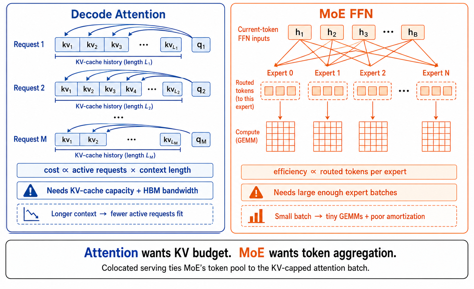
Simply speaking, the decoding phase of an MoE model alternates between two types of layers: the attention layer, which computes the attention operation with KV cache, and the MoE layer, which routes each token in the batch to a small set of experts. When the requests become longer, the KV caches of each requests also grows, saturating the GPU memory capacity. In general, calculating attention requires KV cache to be presented in GPU memory. Therefore when the workload contains requests with longer-context length, the batch size that the system can forward in one iteration become smaller. This smaller batch directly hurts the MoE layer. With fewer active tokens, fewer routed tokens reach each expert, making the expert GEMMs smaller and less efficient, causing MoE utilization to drop.
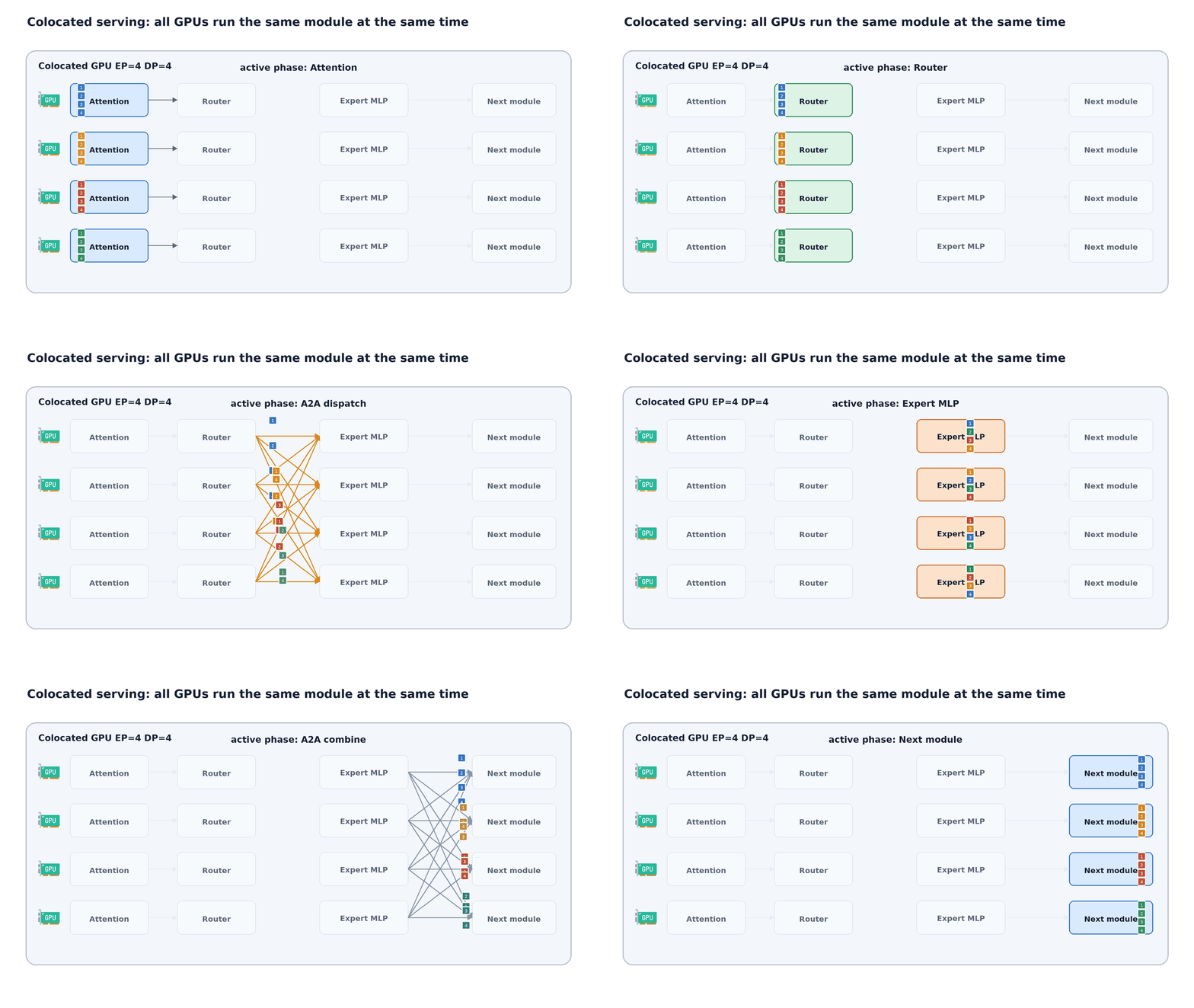
This mismatch creates a fundamental tension in colocated MoE serving: a colocated MoE serving layout runs attention and the MoE layer on the same workers. Each worker keeps KV cache for its active requests, runs attention, computes routing, participates in expert-parallel dispatch, executes local experts, combines expert outputs, and then advances to the next module. Figure 2 shows this layer-by-layer flow. The key consequence is that the requests admitted for attention also define the token pool available to MoE. That coupling is harmless only if the attention-selected batch is also large enough for efficient expert execution.
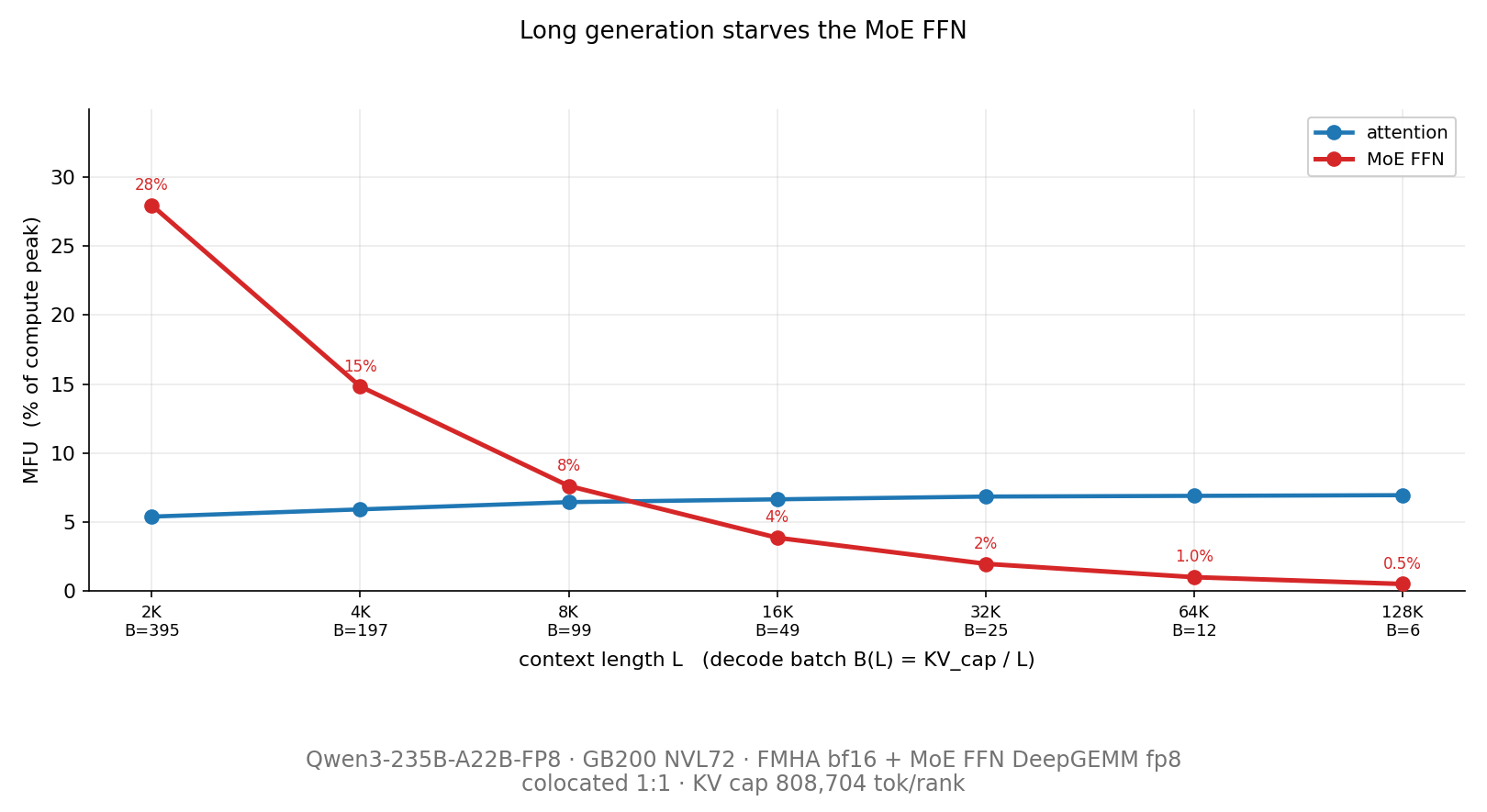
When serving requests with long-context, the decode phase exposes a utilization imbalance in colocated MoE serving: the KV-capped batch starves the MoE FFN, while attention remains roughly steady. We measure this split using model FLOPs utilization (MFU), normalized to the hardware compute peak of each operator. Figure 3 fixes the per-rank KV-cache budget and reduces the decode batch as context length grows, so that the total resident KV history per rank stays roughly constant. This control separates KV-cache capacity from batch-size effects. Decode attention is HBM-memory-bound, so reading a similar amount of KV cache from HBM keeps its MFU nearly flat. MoE FFN, however, is dominated by expert GEMMs on the current decode batch. As context length grows, the active batch shrinks, so fewer routed tokens enter the MoE layer. Each local expert receives fewer tokens, its GEMM becomes smaller, and MFU drops because expert-weight reads, routing, dispatch, and kernel overhead are amortized over less GEMM work.
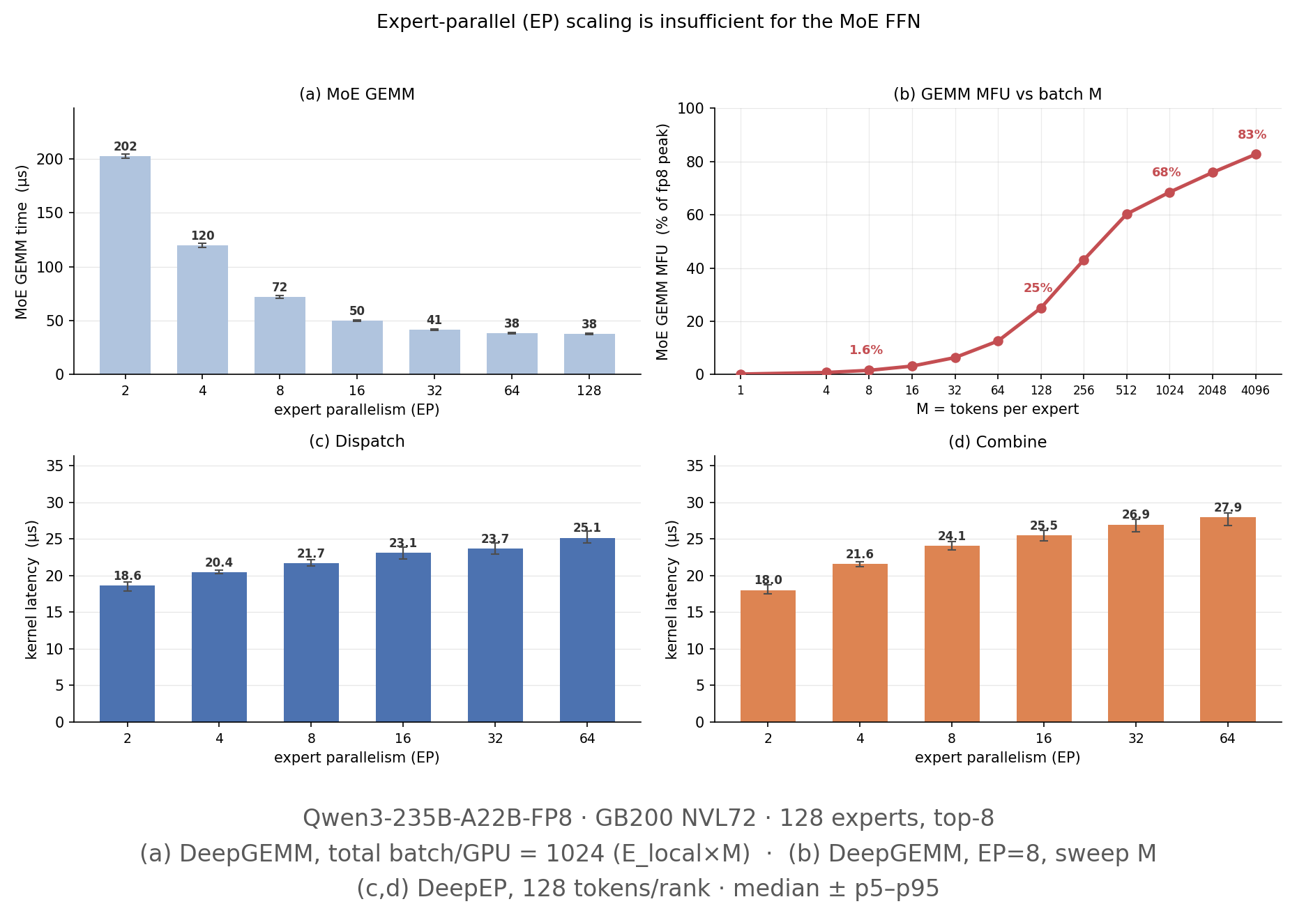
Increasing EP reduces expert-weight traffic, but it does not change MoE compute. EP mainly changes how much expert-weight memory traffic each GPU pays from HBM; it does not change how many tokens the colocated batch sends into MoE. In a colocated run, the active batch is already fixed by attention admission. Once that batch is fixed, the MoE layer receives a fixed routed-token pool. With balanced routing, changing EP repartitions that pool across GPUs but leaves per-GPU expert FFN FLOPs roughly unchanged. What changes is local expert ownership: each GPU stores and loads fewer expert-weight matrices from HBM, and its routed tokens are grouped over fewer local experts.
Figure 4 shows why EP helps only until local expert-weight traffic stops dominating, and why it cannot fix the MoE batch shortage. Panel (b) is batch scaling: it keeps local expert ownership fixed and increases the per-GPU MoE token count. More tokens per local expert make the GEMMs larger, so MFU rises sharply. Panel (a) is EP scaling: it keeps the per-GPU MoE token count fixed and increases EP, which reduces local expert ownership. Per-GPU expert FFN FLOPs stay roughly unchanged, but each GPU loads fewer expert-weight matrices from HBM and runs fewer, larger local expert GEMMs. Latency falls at first, then stabilizes once expert-weight traffic is no longer the bottleneck. Panels (c) and (d) show that dispatch and combine remain in the path. EP therefore has diminishing returns: it reduces local memory traffic, but it does not raise per-GPU MoE token count or remove communication. Perplexity’s Qwen-on-Blackwell report observes the same pattern, with diminishing returns after sharding 128 experts across more than 16 ranks on Blackwell [4].
These observations reveal a fundamental tension in MoE inference. The attention side should use its KV-cache budget to keep the active request batch as full as possible; its MFU is much less sensitive to the resulting batch-size tradeoff. However, the FFN side must aggregate routed tokens beyond what any one attention worker can admit, because MoE MFU falls when each local expert receives too few tokens. We next describe the Attention-FFN Disaggregation (AFD) placement pattern from MegaScale-Infer and Step-3, which separates these two placement decisions instead of trying to satisfy both with one colocated batch [1] [2].
Disaggregating Attention and FFN
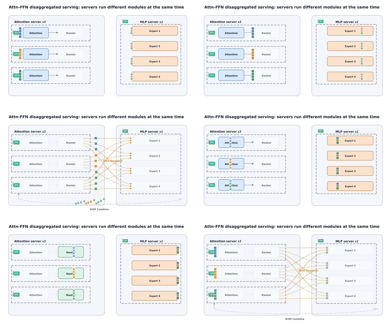
Following prior AFD work such as MegaScale-Infer and Step-3, Attention-FFN Disaggregation changes placement, not model computation [1] [2]. Attention workers keep the request-facing path: KV cache, attention, routing, and sampling. FFN workers receive routed tokens, execute the MoE FFN, and return the layer outputs. For each layer, the attention-side router produces expert assignments, and the routed-token batch becomes the boundary between attention-side decode and FFN-side execution.
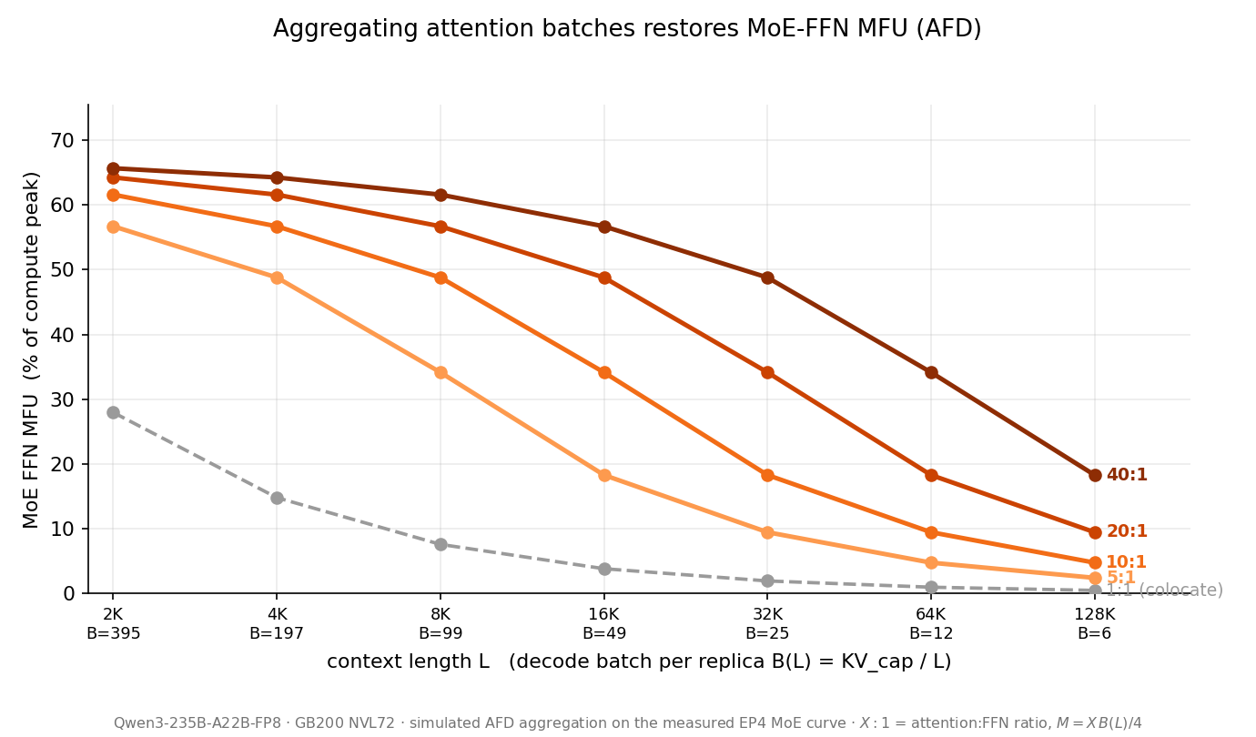
This boundary addresses the coupling from the colocated layout. Attention admission can remain governed by KV-cache capacity and target context length. The FFN side no longer depends on one attention worker’s KV-limited batch; it aggregates routed tokens from multiple attention workers before running grouped expert GEMMs. With the FFN-worker pool fixed, aggregation increases the routed-token batch seen by each local expert. Figure 5 shows the effect: increasing the number of attention workers feeding the same FFN pool lifts MoE MFU above the colocated baseline.
Attention worker. An attention worker owns request state and request progression. It keeps scheduler-visible request state, KV cache, QKV and output projections, KV-cache attention, residual/norm state, the MoE router, and sampling. Compared with the FFN worker, it holds only a small fraction of the model weights. For each layer, it computes attention over its local KV cache, routes the current tokens, and packs the routed tokens for dispatch to the FFN side. After the final layer returns, it samples the next token and continues the sequence.
FFN worker. An FFN worker owns the weight-heavy MoE path, but not request state. For the large MoE checkpoints we evaluate, most model weights are expert weights (>90% parameters), so FFN workers store the expert weights and execute the MoE computation. They receive routed tokens from attention workers, group tokens by expert, run expert GEMMs and activations, combine the selected expert outputs, and send the layer outputs back. The FFN worker does not own KV cache, request progression, routing decisions, or sampling.

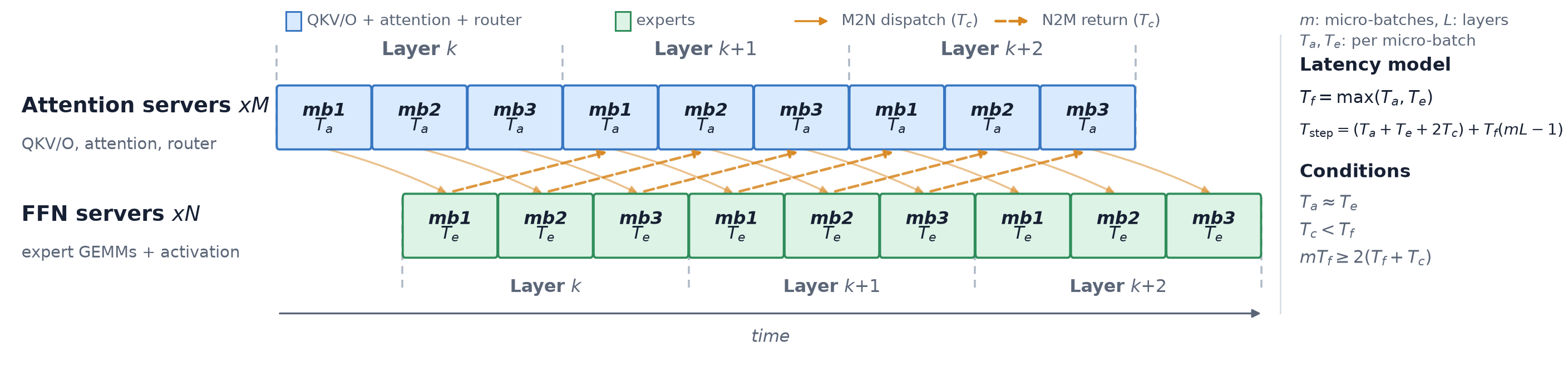
AFD trades MoE batch aggregation for cross-role token movement. Following MegaScale-Infer’s notation, we write $M$ for the number of attention nodes and $N$ for the number of FFN nodes [1]; on the GB200 NVL72 rack used in our evaluation, each node hosts four workers, one per GPU. In every transformer layer, attention workers send routed tokens to FFN workers through M2N dispatch, and FFN workers return expert outputs through N2M combine. If this boundary is serialized, every layer pays dispatch and combine on the critical path, which can erase the gain from larger expert batches. A practical AFD runtime therefore has to pipeline the boundary: split the decode batch into microbatches, let the MoE side execute one microbatch while the attention side advances another, and overlap M2N/N2M traffic with compute instead of treating communication as a separate stage.
MegaScale-Infer gives an idealized three-condition model for this pipeline. Figure 7 follows its notation: $m$ microbatches and $L$ MoE layers. For one microbatch at one layer, $T_a$ is the attention-side compute time, $T_e$ is the MoE-side compute time, and $T_c$ is the one-way communication time. The steady-state microbatch period is $T_f=\max\{T_a,T_e\}$. Under this model, the global-batch decode-step latency is $T_{\text{step}} = (T_a + T_e + 2T_c) + T_f(mL - 1)$. The model says an ideal ping-pong pipeline keeps both sides busy when three conditions hold: (1) attention and MoE compute are balanced ($T_a \approx T_e$); (2) one-way communication is shorter than the pipeline period ($T_c < T_f$); and (3) the number of microbatches is large enough to hide both communication directions ($mT_f \geq 2(T_f + T_c)$). We use these conditions as an analytical reference, then test which ones are actually binding in our GB200 measurements.
GB200 NVL72 provides the hardware conditions that AFD needs, but it also makes the colocated baseline stronger. NVIDIA describes GB200 NVL72 as a rack-scale system with 36 Grace CPUs and 72 Blackwell GPUs in one 72-GPU NVLink domain, organized as 18 compute nodes with 4 Blackwell GPUs each. Each Blackwell GPU has 192 GB of HBM3e, and the rack provides 720 PFLOPS of sparse FP8/FP6 Tensor Core compute, 13.4 TB of HBM3e with 576 TB/s aggregate HBM bandwidth, and 130 TB/s of NVLink bandwidth across the rack [3]. NVIDIA also highlights 1.8 TB/s GPU-to-GPU interconnect per GPU through fifth-generation NVLink [3]. These hardware numbers cut both ways. The rack-scale NVLink/NVSwitch bandwidth makes AFD practical because routed tokens can move quickly between attention and FFN workers. At the same time, Blackwell FP8 compute and HBM bandwidth make the colocated baseline stronger, so AFD has to hide communication and runtime overhead rather than relying on disaggregation alone. Perplexity’s Blackwell Qwen deployment report makes the same point from the colocated side: with a full NVL72 rack, high intra-rack bandwidth and wide expert parallelism can already make colocated MoE serving highly competitive [4].
FastAFD: Building an Attention-to-FFN Runtime on GB200 NVL72
The previous sections argue that AFD is the right placement. Whether it pays off on GB200 NVL72 depends on the runtime, because the colocated baseline is already strong on this hardware. Three costs decide the outcome: M2N/N2M communication that would otherwise sit on every layer’s critical path; launch and synchronization overhead across the many small stages of a decode step; and a cluster-wide control plane that must produce a plan for every decode step.
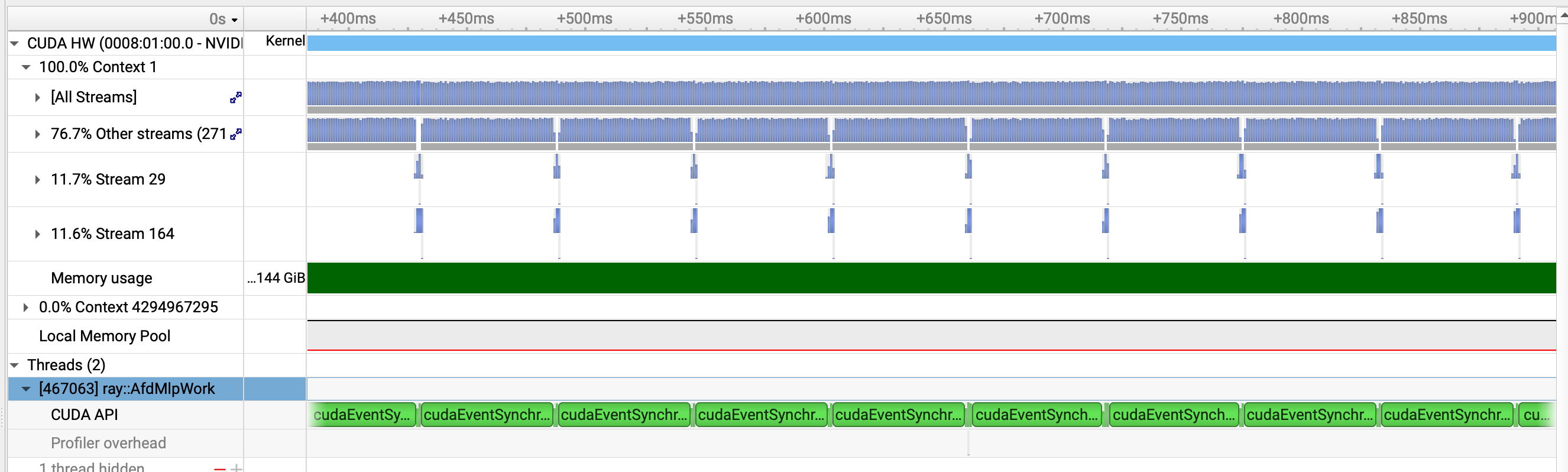
FastAFD implements AFD as a role-specialized runtime built on Mini-SGLang, a compact serving engine distilled from SGLang [10]. Ray launches attention workers, FFN workers, and one logical coordinator; each 4-GPU node hosts four workers, one per GPU. Attention workers run the request-facing transformer path: QKV and output projections, KV-cache attention, KV updates, residual/norm state, the MoE router, and sampling. FFN workers own the expert path: they receive routed tokens, execute the experts, and send layer outputs back. The coordinator builds a plan for each decode step: which requests are active, which microbatch and buffer slots each rank uses, and which attention and FFN peers participate in the step.
Each optimization targets one of these costs. To keep communication off the critical path, FastAFD adapts DeepEP dispatch/combine to the asymmetric M2N/N2M pattern, so routed tokens move through GPU-side kernels over NVLink/NVSwitch instead of a CPU-driven transport stack; a microbatch pipeline then overlaps this traffic with attention and FFN compute. To cut launch and synchronization overhead, a MegaMoE-inspired path fuses token grouping, packing, dispatch/combine handling, expert GEMMs, and activation into one FFN-side kernel, and CUDA graphs capture the rest of the decode path. To hide the control plane, the coordinator follows SGLang’s zero-overhead scheduler: it prepares the next step-level plan while workers replay the current CUDA graph. The rest of this section examines each mechanism.
Keeping the M2N/N2M Control Path on the GPU
AFD communication is bipartite and asymmetric. During M2N dispatch, attention ranks (one rank per attention worker) send routed tokens to FFN ranks; during N2M combine, FFN ranks return layer outputs to the corresponding attention ranks. Prior AFD systems and FastAFD place the control path of this boundary differently, and the difference follows from their fabrics.
MegaScale-Infer and Step-3 both connect attention and FFN workers through an inter-node RDMA fabric, and both keep the communication control path on CPUs. MegaScale-Infer drives M2N transfers from an in-house CPU library: CUDA events and driver operations gate the GPU stream, a CPU-side sender issues RDMA write-with-immediate and polls completions, and the receiver polls completions and issues a GDRCopy flush for GPU-visible consistency [1]. StepMesh, Step-3’s communication library, builds worker/server push-pull APIs on BytePS: dedicated network threads execute RDMA operations on CPUs, while GPUDirect RDMA keeps tensor payloads in GPU memory [6]. This choice has a stated benefit: communication consumes no GPU SMs, which MegaScale-Infer cites as a reason to avoid GPU-side schemes.
FastAFD targets a different fabric. On GB200 NVL72, attention and FFN workers share one NVLink/NVSwitch domain, so the boundary is intra-rack GPU-to-GPU token movement, and FastAFD keeps both payload and control on the GPU by reusing DeepEP’s dispatch/combine kernels [7]. DeepEP assumes a symmetric EP world in which every rank owns experts. A thin adapter maps AFD onto that contract instead of modifying it: it forms one process group over all attention and FFN ranks, assigns each attention rank a block of dummy expert slots that the router never selects, and remaps real expert ids into the FFN ranks’ slot range before dispatch. Attention ranks therefore only send during dispatch and only receive during combine; FFN ranks do the reverse. Dispatch and combine run as GPU kernels with event-based synchronization, no CPU post/poll sits on the decode critical path, and the boundary stays compatible with CUDA-graph capture of the decode step. The trade-off is the one MegaScale-Infer avoided: GPU-side communication spends SMs. The next subsection shows how FastAFD turns that cost into overlap by fusing the transfers into the expert kernels themselves.
MegaMoE: Fusing Dispatch, Expert Compute, and Combine
In decode, the cost of an MoE layer is not only the expert GEMMs. The runtime must use the router’s top-k decisions to pack tokens for remote experts, move those token buffers, run the expert projections and activation, combine the selected expert outputs, and scatter the result back to the original token order. Implemented as separate kernels and communication launches, each boundary materializes intermediate buffers and routing metadata, adds events or stream synchronization, and gives the system only coarse places to overlap communication with compute. These fixed costs are especially visible in decode, where per-expert batches are small and imbalanced. DeepGEMM’s MegaMoE removes these boundaries within one MoE layer: it fuses EP dispatch, the expert GEMMs with SwiGLU, and EP combine into a single kernel that moves tokens through symmetric memory over NVLink while Tensor Cores compute [8]. This is also what repays the SM cost of GPU-side communication from the previous subsection: the transfer instructions live inside a kernel that is computing at the same time, so communication fills gaps instead of occupying stages.
The upstream kernel is symmetric: every rank both contributes tokens and owns experts. At the AFD boundary the roles are disjoint, so FastAFD splits the mega-kernel into two role kernels. The attention-side kernel is one fused launch per layer and microbatch: it quantizes hidden states to FP8, publishes routing metadata so FFN ranks can pull the payload, waits for the expert write-back, and reduces the top-k expert outputs into the layer output. It occupies 24 of a Blackwell GPU’s 148 SMs, leaving the rest to the attention path running concurrently. The FFN-side kernel pulls FP8 tokens from all attention ranks, runs the grouped expert GEMMs with SwiGLU fused into the GEMM pipeline, and pushes BF16 outputs back into each source rank’s combine buffer. All movement is one-sided through pre-allocated symmetric buffers, with no per-transfer handshake; tokens cross the boundary as FP8 and return as BF16, which is where the roughly 3 bytes per hidden element in the communication estimate later in this post comes from.
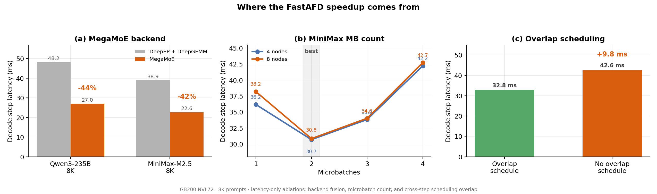
Role specialization then allows a fusion that a colocated layout could not support: because an FFN worker runs nothing but this receive-compute-return loop, FastAFD launches one persistent FFN-side kernel per decode step. It owns the whole GPU, serves every MoE layer and every microbatch lane, and reads each layer’s weights from a descriptor table, so per-layer and per-microbatch launches disappear from the FFN side entirely. The attention side intentionally stays per-layer: attention ranks still run KV-cache attention, KV updates, and residual/norm work between boundaries, so their boundary work remains the single fused kernel above. The current kernels assume uniform expert shapes across layers, 512-aligned hidden and intermediate sizes, and at most four microbatch lanes, which is sufficient for the evaluated checkpoints but a real constraint for broader model coverage. Figure 13, in the ablation subsection, quantifies the fusion: it reduces 8-node decode-step latency by 44% on Qwen3-235B and 42% on MiniMax-M2.5 relative to the separate-stage DeepEP + DeepGEMM path.
Scheduling Away the Control Plane
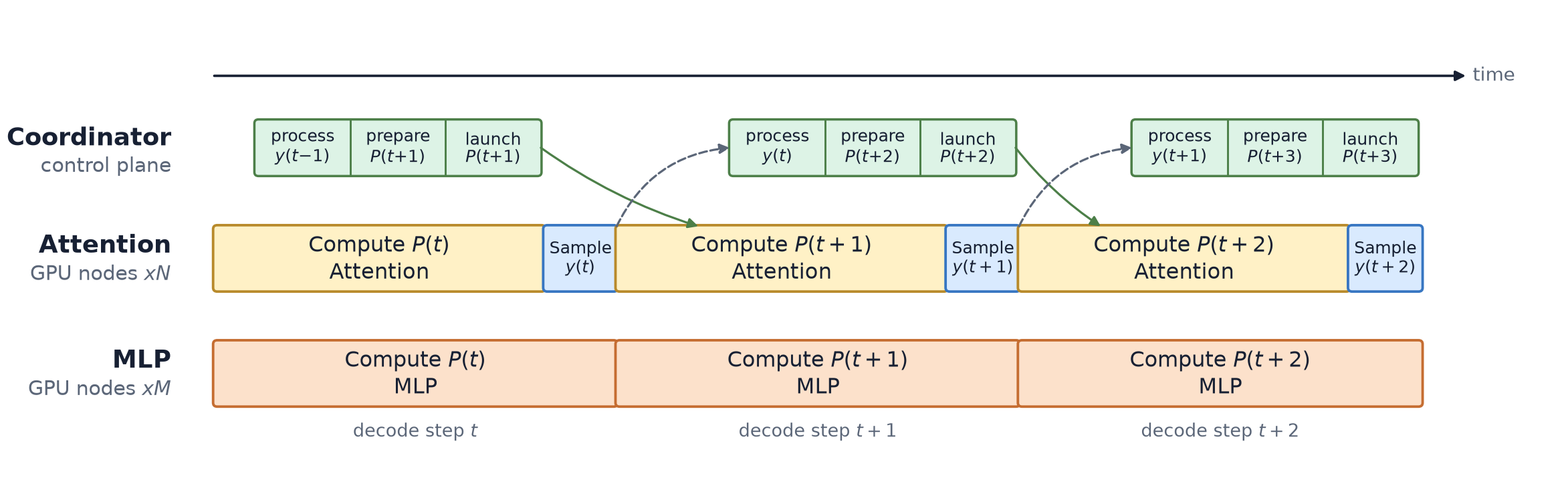
With multiple attention and FFN workers spread across nodes, AFD is usually a cross-node system rather than a single-node data-path optimization. Every decode step needs a CPU-side plan: which requests are active, how the batch is padded and split into microbatches, which graph bucket and buffer slots each rank should use, which attention and FFN peers participate, and which KV-cache table entries can be freed. The coordinator does not compute routing or drive the dispatch/combine data path; those stay on the workers and GPU streams. The CPU control path is still slow enough that FastAFD must hide it behind GPU execution instead of placing it between decode steps.
The idea follows SGLang’s zero-overhead scheduler: CPU-side scheduling runs one step ahead while GPUs execute already-prepared metadata [9]. The difference is that FastAFD uses one coordinator that owns scheduling for all attention workers and manages the attention/FFN workers across nodes. At each decode step, the coordinator processes returned sampled tokens, prepares the next step-level plan, and publishes that plan through ZMQ while workers run the current plan. ZMQ does not carry routing decisions or data-path work: router top-k, token packing, M2N dispatch, FFN execution, and N2M combine all run inside the worker GPU path. ZMQ only carries control commands and returned sampled tokens. This removes a cluster-wide scheduling round trip from the decode critical path.
Decode Throughput on Blackwell NVL72
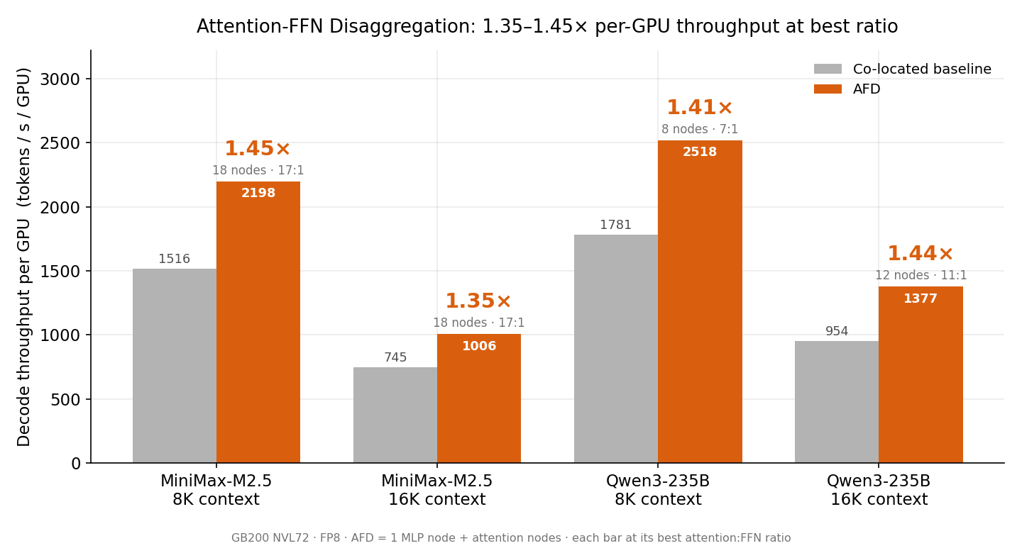
We evaluate FastAFD on steady-state decode, where the AFD boundary is on the critical path of every generated token. The baseline is vLLM in a colocated MoE layout with data parallelism (DP) and expert parallelism (EP), a common reference point for high-throughput LLM serving [5]; the comparison is decode-only, excluding prefill latency and online arrival effects.
The experiments use two open FP8 MoE models:
- Qwen/Qwen3-235B-A22B-FP8: 235B total parameters, 22B activated parameters, 94 layers, 128 experts, and 8 activated experts per token.
- MiniMaxAI/MiniMax-M2.5: an FP8 MiniMax-M2-series model with about 230B total parameters and 10B activated parameters; its public configuration uses 62 layers, 256 local experts, and 8 activated experts per token.
Prompts are random real-text samples from the web, packed to 8K or 16K tokens, and both systems run at a KV-cache memory ratio around 0.85, close to the largest feasible decode batch at each context length. Each GB200 NVL72 rack links 18 nodes, four GPUs each, in one NVLink/NVSwitch domain, so a run with a single FFN node can reach at most 17:1. A FastAFD run uses $M$ attention nodes and $N{=}1$ FFN node: $4M$ data-parallel attention GPUs (tp=1) and 4 FFN GPUs (ep=4), with mb=2 microbatches throughout. The vLLM baseline runs on one 4-GPU node with colocated dp=4, ep=4, DeepEP and DeepGEMM enabled, which was the best EP setting we found. After prefill, we profile a window of synchronized steady-state decode steps; with a fixed batch and CUDA-graph replay, step latency is stable across the window.
The metric is per-GPU decode throughput: tokens generated per step, divided by the step latency and by the total GPU count of the run, including, for FastAFD, the FFN GPUs that host no requests. The vLLM baseline is measured on one node; because colocated DP nodes serve requests independently, its per-GPU throughput is unchanged at larger node counts.
Figure 10 reports the comparison at each workload’s best measured ratio $M{:}N$. Qwen3-235B improves per-GPU decode throughput by 1.41x at 8K and 1.44x at 16K; MiniMax-M2.5 by 1.45x at 8K and 1.35x at 16K. The two models trend in opposite directions with context length: MiniMax falls, and Qwen rises. Both trends, along with why the best ratio stops growing, follow quantitatively from the analysis in the next section.
Where the Speedup Comes From
Per-GPU decode throughput has the same definition for both systems: tokens generated per step, divided by the decode-step latency $T$ and by all GPUs in the run. The two systems place requests differently. In the colocated baseline, every GPU hosts requests; with a resident batch of $B_{\text{vLLM}}$ on each GPU, per-GPU throughput is $B_{\text{vLLM}} / T_{\text{vLLM}}$. Here, resident batch means the number of active requests whose KV cache stays resident on that GPU during decode. In FastAFD, requests live only on the attention side: each of the $4M$ attention GPUs holds a resident batch of $B_{\text{AFD}}$, while the $4N$ FFN GPUs ($N{=}1$ here) hold none yet still count in the denominator. Per-GPU throughput is therefore
$$\frac{4M \cdot B_{\text{AFD}}}{(4M + 4N) \cdot T_{\text{AFD}}}$$Dividing this expression by the colocated baseline gives the speedup as a product of three factors:
$$\text{speedup} \;=\; \underbrace{\frac{B_{\text{AFD}}}{B_{\text{vLLM}}}}_{\text{batch expansion}} \;\times\; \underbrace{\frac{T_{\text{vLLM}}}{T_{\text{AFD}}}}_{\text{latency ratio}} \;\times\; \underbrace{\frac{M}{M+N}}_{\text{FFN-node tax}}$$Each factor has a distinct origin. Batch expansion comes from memory capacity: a colocated GPU holds its ep=4 expert shard, the dense weights, and KV cache, while a FastAFD attention GPU holds only the non-expert weights, a small fraction of the checkpoint, leaving the rest of its memory for KV cache and hence a larger resident batch at the same context length. The FFN-node tax, our name for the factor $M/(M+N)$ from the derivation, is fixed by topology: FFN GPUs contribute to every generated token but host no requests. Both factors are thus set before a single step runs, and the identity is exact by construction. That leaves the latency ratio $T_{\text{vLLM}} / T_{\text{AFD}}$. The direct way is to measure both step periods. The next subsection instead computes $T_{\text{AFD}}$ from the vLLM run alone: the step decomposition gives the attention-side work that remains after disaggregation, and the memory budget gives the AFD batch size.
Predicting the GB200 speedup
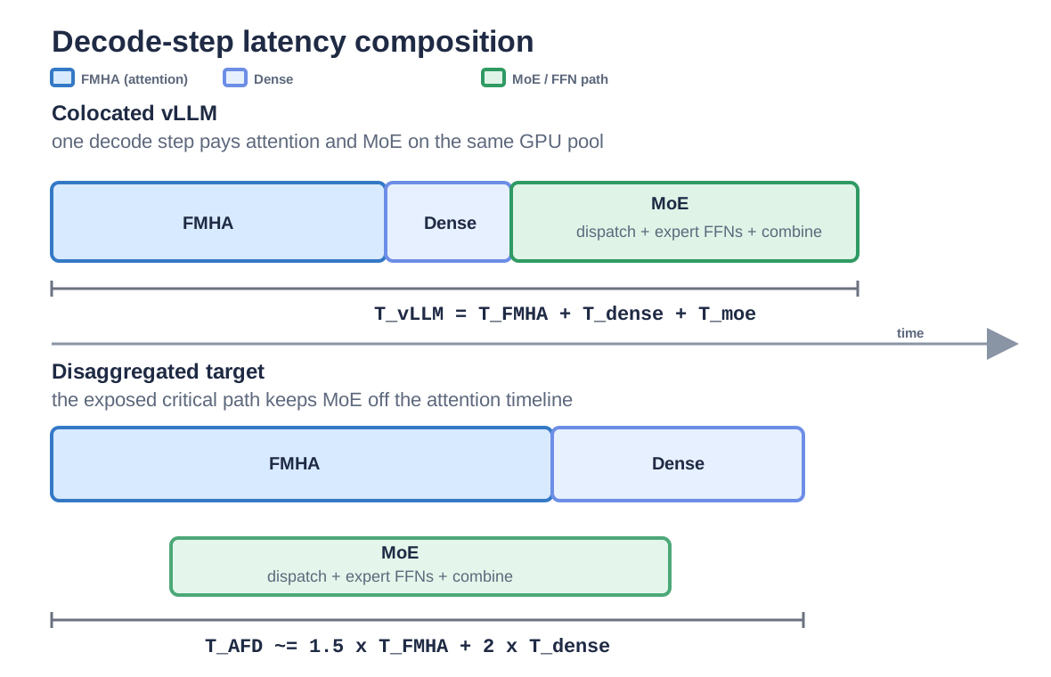
This subsection works under what we call the hidden-FFN condition, written $T_e \le T_a$ in the notation of the microbatch model above: attention work fully covers MoE execution and M2N/N2M communication, so the FastAFD decode-step period equals the attention-side period. When the FFN side is exposed instead ($T_e > T_a$), it sets the step period and this predictor does not apply. The inequality deliberately replaces condition (1) of that model, MegaScale-Infer’s balance target $T_a \approx T_e$; the regime analysis below shows why. Note the change of scale: $T_a$ and $T_e$ are per-layer microbatch times, while $T_{\text{vLLM}}$, $T_{\text{AFD}}$, and the components below are whole-step periods, the same work summed over all layers and microbatches. Under the hidden-FFN condition, $T_{\text{AFD}}$ is the attention side of the pipeline end to end, and we predict it from the vLLM step decomposition measured on GB200 (Figure 11). $T_{\text{moe}}$ collects what AFD removes from the attention critical path: expert GEMMs, activation/quant, dispatch, and combine. The work that stays on the attention workers has two parts: the fused multi-head attention kernel (FMHA, with time $T_{\text{FMHA}}$), and $T_{\text{dense}}$, which collects dense projections, routing, norms, KV-cache updates, quant/cast, and small kernels. The step is thus $T_{\text{vLLM}} = T_{\text{FMHA}} + T_{\text{dense}} + T_{\text{moe}}$.
$T_{\text{FMHA}}$ and $T_{\text{dense}}$ are measured at vLLM’s operating point, and FastAFD runs at a different one: a larger resident batch, split into two microbatches. The batch is larger because an attention GPU no longer stores expert weights; the freed memory holds more KV cache, so the resident batch grows until it fills KV capacity again. At the same context length, this capacity ratio, the batch expansion $B_{\text{AFD}} / B_{\text{vLLM}}$ of the identity, is 1.5x in all four workloads: Qwen fits 96 requests per attention GPU versus vLLM’s 64 at 8K and 48 versus 32 at 16K; MiniMax fits 72 versus 48 at 8K and 36 versus 24 at 16K.
The two parts respond to this operating point differently. FMHA is one large HBM-bound kernel whose time tracks the KV bytes it reads: a 1.5x resident batch means 1.5x KV traffic, so $T_{\text{FMHA}}$ scales by 1.5x. $T_{\text{dense}}$ is mostly small kernels, too small for a larger batch to amortize their fixed costs. Their time tracks launch count rather than batch size, and they run once per microbatch, so this part scales with the microbatch count $m$ (mb=2 in all measured runs):
$$T_{\text{AFD}} \;\approx\; \frac{B_{\text{AFD}}}{B_{\text{vLLM}}} \cdot T_{\text{FMHA}} \;+\; m \cdot T_{\text{dense}}$$This formula also explains why, once communication is fully hidden, fewer microbatches are better: extra microbatches mostly add another copy of the small-kernel term.
Substituting the predictor into the identity, with the measured $B_{\text{AFD}} / B_{\text{vLLM}} = 1.5$, $m = 2$, and $N = 1$, gives
$$\text{speedup} \;=\; 1.5 \times \frac{T_{\text{vLLM}}}{1.5 \cdot T_{\text{FMHA}} \,+\, 2 \cdot T_{\text{dense}}} \times \frac{M}{M+1}$$The remaining terms are all external to FastAFD measurement: $T_{\text{vLLM}}$, $T_{\text{FMHA}}$, and $T_{\text{dense}}$ are read from the vLLM step decomposition, and $M$ is the topology choice. We validate the prediction at each workload’s best measured topology from Figure 10: 17:1 for MiniMax at both context lengths, 7:1 for Qwen at 8K, and 11:1 for Qwen at 16K. While the FFN side stays hidden, the predicted attention-side period does not depend on $M$; only the tax changes with topology.
| Workload | Measured speedup | Predicted speedup |
|---|---|---|
| MiniMax-M2.5 8K | 1.45x | 1.45x (+0.0%) |
| MiniMax-M2.5 16K | 1.35x | 1.38x (+2.2%) |
| Qwen3-235B 8K | 1.41x | 1.41x (+0.0%) |
| Qwen3-235B 16K | 1.44x | 1.44x (+0.0%) |
The measured GB200 speedup is reproduced workload by workload. The identity adds no error of its own: the capacity ratio is measured and the tax is set by node counts, so the residuals come entirely from $T_{\text{AFD}}$, whose step-period prediction itself agrees with the Nsight Systems replay periods to within 2%. The agreement holds only while the FFN side stays hidden ($T_e \le T_a$), the condition the next subsection examines.
When does the FFN side stay hidden?
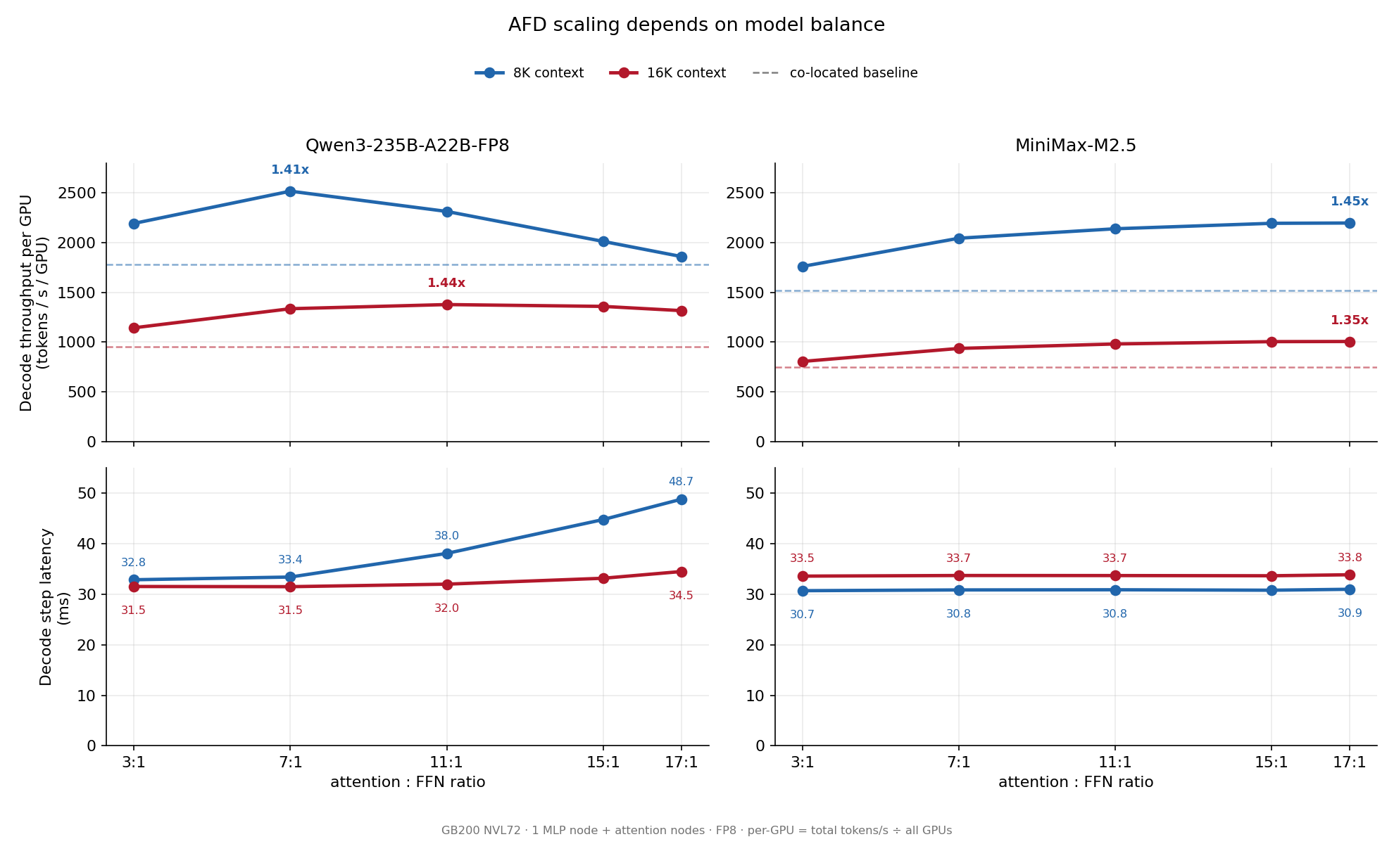
The predictor rests on one condition: the FFN side stays hidden ($T_e \le T_a$). Figure 12 shows when that holds and what each side of the boundary costs. It sweeps the ratio $M{:}N$ for both models, with per-GPU throughput on top and the decode-step latency that creates it below. At a fixed context length both systems fill their KV cache, and decode attention is dominated by reading that resident history, so the attention-side time $T_a$ is similar for the two models. What differs is the FFN-side time $T_e$: whether one FFN node can process the routed tokens from $M$ attention nodes while staying hidden behind attention work.
While the FFN side stays hidden ($T_e \le T_a$), the condition is cheap. Attention-side work is unchanged by FFN-side slack, so $T_{\text{AFD}}$ does not grow with $M$, and the only cost of the underutilized FFN node is the tax $M/(M+1)$, a cost that shrinks as $M$ grows, from 12.5% of the GPUs at 7:1 to 5.6% at 17:1. Per-GPU throughput therefore rises with every added attention node. MiniMax-M2.5, with about 10B activated parameters per token, stays in this regime across the measured range: step latency nearly flat, throughput rising through 17:1. Once $T_e > T_a$, the price changes in kind: the FFN node sets the step period, $T_{\text{AFD}}$ grows with $M$ because the routed-token load does, and the latency ratio now falls faster than the tax improves. Qwen3-235B, with 22B activated parameters per token, crosses this boundary inside the sweep: past its best ratio, step latency rises, especially at 8K, where the larger per-attention-GPU batch sends more routed tokens per step, and per-GPU throughput falls.
This asymmetry settles the placement rule. The two failure modes are priced differently: staying hidden wastes at most one node in $M+1$ of FFN capacity, a bounded and shrinking cost, while exposure slows every decode step, a cost that grows with $M$. MegaScale-Infer’s balance target $T_a \approx T_e$ sits exactly on the boundary between the two, and a fixed placement cannot hold that point as batch sizes, context lengths, and model balances shift. Any drift toward $T_e > T_a$ lands in the expensive regime. FastAFD therefore operates at $T_e \le T_a$: the largest $M$ that keeps the FFN side hidden, trading bounded FFN slack for robustness.
What each mechanism preserves
That operating point is cheap to occupy but not automatic to reach. Of the identity’s three factors, the runtime can move only one: memory fixes batch expansion and topology fixes the tax, so every mechanism works through $T_{\text{AFD}}$, either by keeping the FFN side hidden or by keeping the attention-side step free of gaps. The ablations in Figure 13 price each mechanism by removing it. MegaMoE keeps $T_e$ small enough to hide: fusing the separate DeepEP + DeepGEMM stages into one path reduces 8-node decode-step latency by 44% on Qwen3-235B and 42% on MiniMax-M2.5; without the fusion, the FFN side is exposed earlier and the viable $M$ is smaller. Zero-overhead scheduling keeps the step period at its CUDA-graph length: with cross-step overlap disabled, workers wait between replays for the next plan, and the Qwen3-235B 4-node 8K step grows from 32.826 ms to 42.612 ms, a 23% throughput loss that pushes the configuration below the colocated baseline. mb=2 keeps $m$ at its minimum useful value: mb=1 leaves M2N dispatch, FFN execution, and N2M combine exposed on the critical path, while mb=3 and mb=4 raise the $m$-scaled term of the predictor without hiding anything more. MiniMax accordingly reaches its best latency at mb=2 on both 4-node and 8-node runs. This is also the measured answer to conditions (2) and (3) of the microbatch model: on this fabric the one-way transfer fits under the pipeline period ($T_c < T_f$), and $m{=}2$ already meets the hiding requirement.
With the identity validated term by term, projecting heterogeneous hardware reduces to a substitution: remove the FFN-node tax, and remove MoE time from the latency ratio. The next section applies this substitution to Vera Rubin + LPX/LPU.
What Would Vera Rubin + LPX/LPU Change?
Vera Rubin + LPX/LPU turns AFD from a GPU placement problem into a hardware boundary. NVIDIA describes Rubin GPUs as the side that handles prefill, decode attention, KV-cache-heavy work, and high-concurrency serving, while LPX accelerates latency-sensitive FFN and MoE execution [17]. Public Rubin material lists each Rubin GPU with up to 288 GB of HBM4, 22 TB/s of HBM bandwidth, and 3.6 TB/s of bidirectional NVLink 6 bandwidth [18]; public LPX material lists a rack of 256 LPUs with 315 PFLOPS of FP8 inference compute, 128 GB of SRAM, 40 PB/s of SRAM bandwidth, and 640 TB/s of scale-up bandwidth [17]. These are exactly the two resources AFD separates.
We do not have this hardware, so the numbers below are projections, anchored by the previous section: the same decomposition reproduces FastAFD’s measured step period and speedup on GB200 to within about 2%. The setup mirrors the GB200 comparison. The baseline is Rubin-only colocated serving, analogous to the vLLM baseline above; the AFD case moves the FFN/MoE path to LPX/LPU while Rubin keeps the request-facing path and KV cache. We assume two LPX racks per Rubin rack (so the FP8 weights fit in LPX SRAM), FP8 rather than FP4 execution, and throughput reported per Rubin GPU without normalizing by LPX cost, power, or accelerator count. In the identity, the move removes the FFN-node tax, shrinks and then cancels batch expansion, and turns the latency ratio into a composition ratio; the subsections below walk through each.
Moving MoE to LPX/LPU
The decomposition is the same as in the previous section: $T_{\text{vLLM}} = T_{\text{FMHA}} + T_{\text{dense}} + T_{\text{moe}}$. If LPX/LPU hides the MoE path, Rubin’s exposed step is $T_{\text{FMHA}} + T_{\text{dense}}$.
Rubin’s larger HBM reduces the capacity gain from removing expert weights: the projected batch expansion drops from about 1.5x on GB200 to about 1.25x. Under a first-order linear attention model, however, a larger batch also proportionally increases attention-side time, so the batch factor cancels in per-Rubin-GPU throughput and the projected speedup reduces to the latency composition alone:
$$\text{speedup} \;\approx\; \frac{T_{\text{FMHA}} + T_{\text{dense}} + T_{\text{moe}}}{T_{\text{FMHA}} + T_{\text{dense}}} \;=\; \frac{1}{1 - \text{MoE fraction}}$$Rather than predict how Rubin changes each kernel ratio, the projection assumes Rubin-only serving keeps the attn:dense:moe composition measured from GB200 vLLM. In the identity, this is the $\infty{:}1$ endpoint of the $M{:}N$ sweep: the tax is gone because LPX racks are not counted in the per-Rubin-GPU denominator, the batch factor has cancelled, and only the latency ratio $T_{\text{vLLM}} / (T_{\text{FMHA}} + T_{\text{dense}})$ remains. The $m$-fold duplication of small kernels from the GB200 predictor is also deliberately absent; the projection assumes an implementation that avoids it, one reason to read the numbers as a boundary rather than a forecast.
| Workload | $T_{\text{FMHA}}$ share | $T_{\text{dense}}$ share | $T_{\text{moe}}$ share | Speedup if MoE hidden |
|---|---|---|---|---|
| MiniMax-M2.5 8K | 43.4% | 16.2% | 40.5% | 1.68x |
| MiniMax-M2.5 16K | 48.2% | 15.3% | 36.4% | 1.57x |
| Qwen3-235B 8K | 41.4% | 15.7% | 43.0% | 1.75x |
| Qwen3-235B 16K | 42.4% | 16.0% | 41.6% | 1.71x |
Two checks support this assumption. First, attention is bandwidth-bound: GB200 vLLM FMHA reaches 80 to 91% of the 8 TB/s per-GPU HBM peak, so the shares carry over as long as attention, dense, and MoE improve by similar factors on Rubin. Second, the shares explain the context-length trend: at a fixed KV budget $B(L) \cdot L$ stays roughly constant, so $T_{\text{FMHA}}$ changes slowly while $T_{\text{moe}} \propto B(L)$ shrinks, and the projected speedup falls with context (1.68x to 1.57x on MiniMax, 1.75x to 1.71x on Qwen).
Feasibility rests on capacity, compute, and transport. Capacity: one LPX rack’s 128 GB of SRAM cannot hold either FP8 checkpoint (roughly 230 GB each), so the reference point is two racks per Rubin rack, with 256 GB of SRAM and 630 PFLOPS of published FP8 compute. Compute: at peak FLOPs, FFN/MoE takes 0.12 to 0.70 ms per step even with the full rack of attention GPUs feeding it; these are estimates, not performance claims, but the margin is wide, and MiniMax was already hidden by a single 4-GPU GB200 FFN node. Transport: the largest case moves about 170 MB per Rubin GPU per step (${\sim}3$ bytes per hidden element: FP8 out, BF16 back) against 3.6 TB/s of NVLink 6, far below the attention step. The binding constraint is software overlap and LPX kernel efficiency, not capacity, compute, or links.
Moving dense work too
The projection above keeps FastAFD’s current split: dense work stays on the GPU, and only FFN/MoE moves. Under this boundary, however, LPX/LPU is idle for most of the step, and Rubin still pays $T_{\text{dense}}$. A more aggressive boundary moves the dense path as well: after attention, Rubin sends the token state to LPX; LPX runs routing, dispatch, expert FFNs, combine, and the next dense/QKV preparation; Rubin receives back the inputs for its next attention step. If this path is fully hidden, Rubin’s exposed step approaches attention-only:
$$\text{dense-offload speedup} \;\approx\; \frac{T_{\text{FMHA}} + T_{\text{dense}} + T_{\text{moe}}}{T_{\text{FMHA}}}$$The cost is a tighter dependency chain: every layer’s dense path now crosses the boundary, with larger payloads than the routed-token traffic of the MoE-only design, and LPX dense kernels must be fast enough. As an absolute check, we scale GB200 attention and dense times by Rubin’s HBM bandwidth ratio (22/8 = 2.75x), take LPX MoE at the peak-FLOP times, and budget LPX dense work at the projected Rubin dense time. LPX still finishes well before the projected Rubin attention step:
| Workload | Projected $T_{\text{FMHA}}$ | LPX MoE | LPX dense budget | Slack under attention |
|---|---|---|---|---|
| MiniMax-M2.5 8K | 5.00 ms | 0.24 ms | 1.86 ms | 2.90 ms |
| MiniMax-M2.5 16K | 5.65 ms | 0.12 ms | 1.80 ms | 3.73 ms |
| Qwen3-235B 8K | 5.41 ms | 0.70 ms | 2.05 ms | 2.66 ms |
| Qwen3-235B 16K | 5.17 ms | 0.35 ms | 1.95 ms | 2.87 ms |
The resulting speedups need no new inputs. Both columns follow from the GB200 composition shares above, with the batch factor cancelling as in the MoE-only case: the MoE-only column is $1 / (1 - \text{MoE share})$, and the Dense+MoE column is $1 / (\text{FMHA share})$.
| Workload | MoE-only | Dense+MoE if fully hidden |
|---|---|---|
| MiniMax-M2.5 8K | 1.68x | 2.31x |
| MiniMax-M2.5 16K | 1.57x | 2.07x |
| Qwen3-235B 8K | 1.75x | 2.42x |
| Qwen3-235B 16K | 1.71x | 2.36x |
This is an upper-bound design point, not the current FastAFD boundary. We keep dense work on Rubin in the main projection out of conservatism: moving it changes the dependency chain and adds boundary traffic, and if that path is not fully overlapped it can erase the benefit. The compute margin, however, suggests this boundary is worth testing once hardware and kernels are available.
Both boundaries share one requirement: the remote path must complete within the Rubin-side work that remains.
$$\begin{aligned} \text{MoE-only:}\quad & T^{\text{LPU}}_{\text{moe}} + T_{\text{transport}} \;\le\; T^{\text{Rubin}}_{\text{FMHA}} + T^{\text{Rubin}}_{\text{dense}} \\[2pt] \text{dense+MoE:}\quad & T^{\text{LPU}}_{\text{dense}} + T^{\text{LPU}}_{\text{moe}} + T_{\text{transport}} \;\le\; T^{\text{Rubin}}_{\text{FMHA}} \end{aligned}$$If the condition holds, the system approaches the corresponding attention-side limit; if FFN execution, dense execution, or transport is exposed, or if Rubin makes colocated MoE much faster than attention, the gain shrinks. The conclusion is not a single forecast but a boundary: AFD is the software interface that lets heterogeneous inference hardware specialize each side without changing the model.
Takeaways
On one NVLink domain, communication belongs on the GPU. FastAFD brings the MegaScale-Infer-style M:N architecture to GB200 NVL72, and the fabric flips the first design choice. MegaScale-Infer keeps the communication control path on CPUs to spare GPU SMs, a sound choice for RDMA-connected fleets. On GB200 the SM budget is less scarce: the attention-side boundary kernel runs on 24 of a Blackwell GPU’s 148 SMs, about 16%, and the FFN-side kernel owns its dedicated GPU by design. The fused dispatch/combine repays that slice with overlap and keeps the whole decode step inside CUDA graphs.
Balance is the wrong target. MegaScale-Infer’s $T_a \approx T_e$ sits on the boundary between a cheap failure mode and an expensive one: FFN slack is bounded by one node in $M+1$, while an exposed FFN side slows every step and worsens as $M$ grows. FastAFD instead runs at $T_e \le T_a$ with the largest $M$ that keeps MoE hidden, trading bounded slack for robustness across batch sizes, context lengths, and model balances.
Two microbatches are enough. On this fabric, mb=2 already hides both communication directions, the measured answer to conditions (2) and (3) of the microbatch model. mb=3 and mb=4 only multiply the small per-microbatch kernels by $m$ while hiding nothing more.
The gain is capacity, not latency. FastAFD’s decode step is about as long as vLLM’s; the latency ratio in the identity stays near 1. What changes is what each GPU holds: attention GPUs shed more than 90% of the weights, carry 1.5x more resident requests, and per-GPU throughput lands 1.35 to 1.45x higher after the FFN-node tax.
Because the speedup is computable from the baseline alone, the projection carries weight. The identity plus the vLLM step decomposition reproduced every measured GB200 speedup. The same arithmetic with the tax removed projects 1.57 to 1.75x on Vera Rubin + LPX/LPU with MoE hidden, and above 2x if dense work moves too, conditional on the same hiding inequality that FastAFD already meets on GB200.
Open Source and Future Work
FastAFD is a serving prototype, not a new model architecture. AFD itself is prior systems work: MegaScale-Infer and Step-3 establish the attention/FFN split as a serving direction [1] [2]. FastAFD’s contribution is an open, inspectable GB200 NVL72 implementation with measured decode-throughput gains over tuned vLLM. This post only profiles steady-state decode steps on GB200 NVL72. It does not claim to solve online arrivals, mixed prefill/decode traffic, SLO-aware admission, request migration, or failure recovery. We plan to release the code and scripts at hao-ai-lab/FastAFD.
Broader model and architecture coverage. The current implementation focuses on full-attention MoE models, specifically Qwen3-235B-A22B and MiniMax-M2.5. The next step is to extend FastAFD to recent open large-MoE families such as DeepSeek, Kimi, Qwen3-Next, GLM, and Stepfun [11] [12] [13] [14] [19]. These models stress both sides of AFD: attention may be full, sparse, sliding-window, or hybrid/linear, while MoE routing changes expert count, activation ratio, load balance, and numerical format.
Production serving composition. A production server has to compose AFD with the rest of the serving stack: prefill/decode disaggregation, speculative decoding, admission control, request migration, runtime metrics, load-imbalance handling, and SLO-aware scheduling [15] [16]. Attention load follows context length and active request count. FFN load follows the number of tokens entering the MoE layer, then routing and expert hot spots decide how that work is distributed across FFN workers. Future schedulers should plan against both KV-cache pressure and expert pressure, not only a static attention-to-FFN node split.
Heterogeneous and next-generation hardware. The Vera Rubin + LPX/LPU section above is a projection, not a measurement. It points to the next validation target: whether the same AFD boundary remains cheap when FFN/MoE execution moves from a GPU worker pool to a different accelerator class [17]. If that boundary holds, AFD becomes a portable way to let KV-cache-heavy attention and weight-heavy FFN execution follow different hardware paths without changing the model.
Acknowledgement
We thank NVIDIA for supporting our development on GB200 NVL72. We thank the Qwen team and MiniMax for creating and open-sourcing Qwen3-235B-A22B and MiniMax-M2.5 to the community. We would like to thank Yibo Zhu and Yonghao Zhuang for providing insightful feedback. FastAFD also builds on the open-source work of the SGLang, vLLM, DeepEP, and DeepGEMM teams, without which a system at this scale would not have been possible to build in the open.
References
- Ruidong Zhu et al., “MegaScale-Infer: Serving Mixture-of-Experts at Scale with Disaggregated Expert Parallelism,” arXiv:2504.02263, 2025. https://arxiv.org/abs/2504.02263
- StepFun Team, “Step-3 is Large yet Affordable: Model-system Co-design for Cost-effective Decoding,” arXiv:2507.19427, 2025. https://arxiv.org/abs/2507.19427
- NVIDIA, “NVIDIA GB200 NVL72.” https://www.nvidia.com/en-us/data-center/gb200-nvl72/
- Perplexity Research, “Hosting Qwen on Blackwell,” May 12, 2026. https://research.perplexity.ai/articles/hosting-qwen-on-blackwell
- Woosuk Kwon, Zhuohan Li, Siyuan Zhuang, Ying Sheng, Lianmin Zheng, Cody Hao Yu, Joseph E. Gonzalez, Hao Zhang, and Ion Stoica, “Efficient Memory Management for Large Language Model Serving with PagedAttention,” SOSP 2023. https://arxiv.org/abs/2309.06180
- StepFun Team, “StepMesh: A High-Performance, Low-Latency Communication Library for Attention-FFN Disaggregation,” GitHub repository, 2025. https://github.com/stepfun-ai/StepMesh
- DeepSeek-AI, “DeepEP: an efficient expert-parallel communication library,” GitHub repository, 2025. https://github.com/deepseek-ai/DeepEP
- DeepSeek-AI, “DeepGEMM: clean and efficient FP8 GEMM kernels with fine-grained scaling,” GitHub repository, 2025. https://github.com/deepseek-ai/DeepGEMM
- SGLang Team, “SGLang v0.4: Zero-Overhead Batch Scheduler, Cache-Aware Load Balancer, Faster Structured Outputs,” LMSYS Blog, 2024. https://www.lmsys.org/blog/2024-12-04-sglang-v0-4/
- LMSYS Org, “Mini-SGLang: Efficient Inference Engine in a Nutshell,” 2025. https://www.lmsys.org/blog/2025-12-17-minisgl/
- DeepSeek-AI, “DeepSeek-V4: Towards Highly Efficient Million-Token Context Intelligence,” Hugging Face model card, 2026. https://huggingface.co/deepseek-ai/DeepSeek-V4-Pro
- Kimi Team, “Kimi Linear: An Expressive, Efficient Attention Architecture,” arXiv:2510.26692, 2025. https://arxiv.org/abs/2510.26692
- Qwen Team, “Qwen3-Next-80B-A3B,” Hugging Face model card, 2025. https://huggingface.co/Qwen/Qwen3-Next-80B-A3B-Thinking
- Z.ai, “GLM-4.6,” model release, 2026. https://huggingface.co/zai-org/GLM-4.6
- Yinmin Zhong, Shengyu Liu, Junda Chen, Jianbo Hu, Yibo Zhu, Xuanzhe Liu, Xin Jin, and Hao Zhang, “DistServe: Disaggregating Prefill and Decoding for Goodput-optimized Large Language Model Serving,” OSDI 2024. https://www.usenix.org/conference/osdi24/presentation/zhong-yinmin
- NVIDIA, “How NVIDIA Dynamo 1.0 Powers Multi-Node Inference at Production Scale,” NVIDIA Technical Blog, 2026. https://developer.nvidia.com/blog/nvidia-dynamo-1-production-ready/
- NVIDIA, “Inside NVIDIA Groq 3 LPX: The Low-Latency Inference Accelerator for the NVIDIA Vera Rubin Platform,” NVIDIA Technical Blog, 2026. https://developer.nvidia.com/blog/inside-nvidia-groq-3-lpx-the-low-latency-inference-accelerator-for-the-nvidia-vera-rubin-platform/
- NVIDIA, “Inside the NVIDIA Vera Rubin Platform: Six New Chips, One AI Supercomputer,” NVIDIA Technical Blog, 2026. https://developer.nvidia.com/blog/inside-the-nvidia-rubin-platform-six-new-chips-one-ai-supercomputer/
- StepFun Team, “Step 3.7 Flash,” Hugging Face model card, 2026. https://huggingface.co/stepfun-ai/Step-3.7-Flash/
Citation
@misc{fastafd2026,
  title  = {FastAFD: Open-Source Large-Scale Attention-FFN Disaggregation on Blackwell NVL72},
  author = {Fu, Yichao and Zhang, Yuxuan and Wang, Ruitian and Chen, Junda and Zhang, Hao},
  year   = {2026},
  url    = {https://github.com/hao-ai-lab/FastAFD},
  note   = {Technical blog and open-source release}
}